
|
| Elliott Sound Products | Attenuator Design |
 Main IndexArticles Index
 Information about the design of multi-step attenuators is very sparse on the Net, but these important circuits are used in voltmeters, ammeters, analogue multimeters and oscilloscopes. There are a couple of examples on the ESP site, with the earliest I published being the Project 16 (P16) audio millivoltmeter. If you do a search for 'attenuator', mostly all you'll find is single-stage attenuators used for RF. You may also come across 'stepped attenuators' that are designed to be used as a volume control in some preamplifiers. The simplest multi-stage attenuator is a pot (potentiometer), but these are uncalibrated, and have poor linearity. They are not useful for metering applications.
Finding anything that describes the process of designing a multi-step attenuator is next to impossible. I'm sure that there is something, somewhere, but I was unable to find any formulae or process to determine the values. I obviously know how to do it, since the Project 16 page shows a couple of examples (as do a couple of other projects), but no-one seems to have published anything describing the design process. The intent of this article is to correct this.
Despite what you'll find on the market, an analogue meter remains the best tool for measuring AC voltages, both within the audio range and for RF. It's easy to see changes, which are displayed as a moving pointer rather than a bunch of digits that change seemingly at random, and averaging by eye is easy. You can't do that with a digital readout, and the impression of precision is usually more of a hindrance than anything else. The only thing that comes close is an LED bargraph, often seen on mixers, and rendered in software in audio recording programs such as Audacity.
When looking at varying signal levels, you're usually after a trend, not an absolute value. Measuring dB with a digital meter is possible if the function is included, but most digital multimeters have poor high frequency response, usually rolling off above 1-2kHz. Some manage higher frequencies, but you need to read the datasheet before you buy if that's your goal. I built my Project 16 audio millivoltmeter many, many years ago, and I have a couple of other (analogue) meters that perform much the same function.
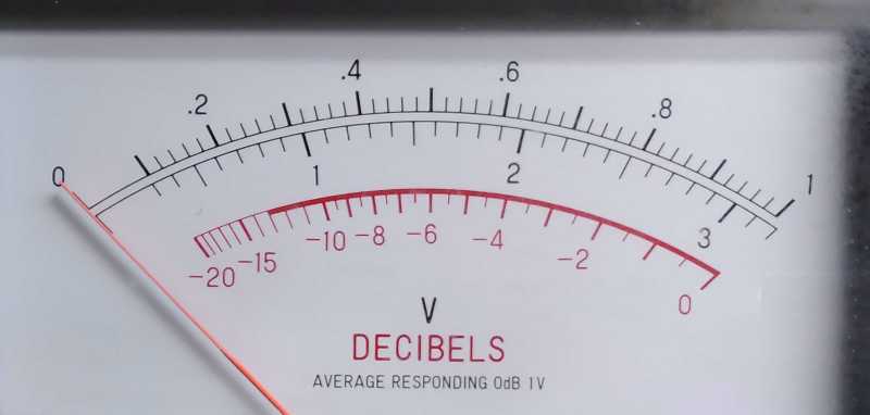
Figure 1.1 - Typical 10dB Step Meter Face
The meter face shown is from a photo of my distortion meter. The different scale lengths are obvious, and this allows a direct reading in 10dB steps. The face also shows that the meter is average responding, but doesn't state that it's RMS calibrated. Most audio millivoltmeters are the same, although ideally they would measure true RMS. The 0dB reference is 1V (0dBV).
Because the step ratio is 1 - 3.16 - 10, the meter has two voltage scales. One uses the full deflection of the meter (10mV, 100mV, etc. steps), and the 3mV, 30mV (etc.) steps will provide full deflection at 3.16, so the scale is either truncated, or it's extended slightly as shown above. This ratio is essential if you need 10dB steps. If the two scales were the same length, you'll get just under 0.5dB error as the switch changes range. All meters that show dB have the same arrangement, and without exception that I'm aware of, all provide 10dB steps.
A common scale for analogue multimeters (for DC voltage) is 100mV, 500mV, 2.5V, 10V, 50V, 250V, 1000V (full scale). While this sequence is not covered in the process described below, it can be determined easily using the same process as any other scale. However, most multimeters just use switched resistors in series with the movement, and that's very easy to calculate once you know the meter's resistance and sensitivity. A typical 20kΩ/Volt meter has a sensitivity of 50µA. The meter movement's internal resistance is only relevant for voltages below 10V DC, and it's irrelevant above that (assuming a basic accuracy of ±3% or so). For example, the 10V range requires a total resistance of 200k, and the movement's resistance will be less than 2k.
Throughout this article you'll see references to the E12 and E24 series for resistors. If you don't know the available values, they are shown in Beginners' Guide to Electronics - Part 1 (Basic Passive Components, section 5.0).
The first step is to work out your specifications. These include the input impedance and the voltage steps required. The latter are determined by usage, and for an oscilloscope the de-facto standard is 1-2-5-10 increments. If you're working with audio voltages, then you'd use 1-3.16-10 steps (10dB ranges). The input impedance depends on preference to an extent, but again, the de-facto standard for oscilloscopes is 1MΩ. Another range is 1-5-10 which is good for voltage measurements (and is the standard for most scopes), but is unusable if you need to read in dB.
There's no standard for analogue multimeters, but these aren't the main topic here. The usual way to describe these is to use kω per volt, as the sensitivity is determined by the meter movement. A basic meter may be rated for 2kΩ/ volt (using a 500µA meter movement), which means that the impedance is 2k for the 1V setting, or 100kΩ on the 50V range. This caused many problems with measurements of high impedance circuits, because the hapless user would see a different voltage displayed depending on the range switch setting. Voltage ranges were often arbitrary due to switch position limitations, largely due to the provision of different measurements (DC volts, AC volts, resistance and milliamps being typical). Modern digital multimeters are usually 10MΩ (or more) input impedance for all ranges.
The first real attempt at making a meter with a constant high impedance input was the VTVM - vacuum tube volt meter. These used a valve stage to buffer and amplify the input. This allowed the input impedance to be much higher than an 'ordinary' meter, and it remained constant regardless of the range selected. FET voltmeters soon followed when 'solid-state' overtook valves as the dominant technology. This meant that there may still be an error (due to the impedance of the measured circuit), but at least it was constant. The input impedance depended on the manufacturer, and was typically between 10MΩ and 20MΩ.
So, the first decision is the input impedance. 1MΩ is always a good start, and that's what will be used for the examples. However, deciding on the impedance without some error margin can (and does) give unobtainable resistor values, so some flexibility is essential. In the first of the examples shown below, I ended up with 1.02MΩ because that gave resistor values that were easily achieved. Having an increase of 20k is not going to create problems, and it's easily corrected with a small gain change in the metering amplifier if needs be.
You may decide on a lower impedance. For example the distortion meter (the meter face is shown in Figure 1) has an input impedance of 100kΩ. This does occasionally cause problems when measuring high impedance circuits, but most 'solid state' gear has low impedances everywhere and the 100k load is of little consequence. The second attenuator example shown is designed for 100k, and this has the advantage that you don't need parallel capacitors provided the stray capacitance can be minimised. More on this later in the article.
Having decided that 1MΩ is a reasonable place to start, we now have to decide on the highest and lowest voltage ranges. The P16 millivoltmeter is designed to cover from 3mV to 30V in 10dB steps. That means that the nominal voltages will be 3mV, 10mV, 30mV, 100mV (etc.). Although the metering amplifier itself isn't covered here, there are several to choose from in the Application Note 002 - Analogue Meter Amplifiers. For a general purpose AC voltmeter, I'll use a range of 3mV to 30V, the same as the P16 circuit. If we want an impedance of 1MΩ the current with full voltage (maximum attenuation) is 30µA (30V / 1MΩ).
The easiest way to determine the resistor network is to start at the top (R1), with the 30V range. The attenuator is calculated backwards, so if we apply the full voltage (31.6V), the output from the 'top' of the attenuator is 31.6V, the next level down is 10V, the next is 3.16V and so on. Essentially, we look at the attenuator with the full voltage applied, and each step is worked out in turn, but in the reverse order.
Since the next voltage is 10V, the voltage difference is 21.6V. The current is 30µA, so the resistor must be 720k - a somewhat 'inconvenient' value (to put it mildly). This isn't a value in any readily available resistor series, so we need to change it. For the sake of this exercise, we'll use 680k, as that's a standard value. The full-range input current is changed, and becomes ...
I = V / R
I = 21.6V / 680k = 31.76470588µA (31.765µA is close enough)
The last resistor in the chain (R9, see drawing below) is expected to provide 3mV output with an input voltage of 31.6V at 31.765µA, so it must be ...
R = V / I
R = 3.16mV / 31.765µA = 99.48Ω
In this case we'd use 100Ω, which is so close it doesn't matter. The error is well below 1%, and can be ignored.
Now we can work out the nest resistor in the sequence (R2). We know the current and can easily work out the voltage difference between 10V and 3.16V, as this is the voltage across R2 ...
R = 6.84V / 31.765µA = 215.33kΩ (we'll use 215kΩ, easily made up with 200k + 15k)
After that, it's simple repetition, with each lower range using the same bases (6.8 and 2.15) divided by 10, and the lowest value in this sequence is 215Ω. The same procedure is used for any number of steps. First, work out the approximate input impedance required. Next, determine the first resistor value, and adjust as needed to get a resistance that's possible. Then, re-calculate the input current so that the last resistor in the attenuator can be calculated, and then determine the second resistor value.
For the attenuator we just designed, the maximum voltage is 31.6V, and the current is 31.765µA. The input impedance is therefore ...
R = 31.6 / 31.765µA = 994.81kΩ
This is a little lower than we wanted, so we'll include R0, with a value of 5.6kΩ, giving a nominal input impedance of 99.94k which is such a small error from 1MΩ that it's not worth worrying about.
Figure 2.1 - Basic Attenuator Circuit, 10dB Steps, 1MΩ
The attenuator shown is accurate to better than 0.05dB across the ranges, and doesn't require any 'special' resistor values. The 200, 2k, 20k and 200k resistors are from the E24 series, and these are readily available from most suppliers worldwide. The standard tolerance will be 1%, but you can select the values to be closer than that if you wish. While the procedure described is somewhat tedious, there's nothing hard about it. If you intend to mess around with stepped attenuators it's worth your while to set up a spreadsheet using OpenOffice or similar.
| Rx | Voltage | Difference | Resistance | Closest R | Check |
| R1 | 31.6 | 21.6 | 680,004.41 | 680,000 | 21.6 |
| R2 | 10.0 | 6.84 | 215,334.73 | 215,000 | 6.82 |
| R3 | 3.16 | 2.16 | 68,000.44 | 68,000 | 2.16 |
| R4 | 1.00 | 0.684 | 21,533.47 | 21,500 | 0.682 |
| R5 | 0.316 | 0.216 | 6,800.04 | 6,800 | 0.216 |
| R6 | 0.100 | 0.0684 | 2,153.35 | 2,150 | 0.0682 |
| R7 | 0.0316 | 0.0216 | 680.00 | 680 | 0.0216 |
| R8 | 0.0100 | 0.00684 | 215.33 | 215 | 0.00682 |
| R9 | 0.00316 | 0.00316 | 99.48 | 100 | 0.00317 |
| Target Current | 31.7645 | µA | Total R | 994,445 | (31.7765µA) |
In the table, the 'difference' column is the voltage shown on that row minus the voltage on the next row. For example, in the first row, the voltage is 31.6V and the difference is therefore 31.6 - 10, which is 21.6V. The resistance is calculated from the difference voltage and the current, and the 'check' column multiplies the selected resistance by the actual current (yellow cell, determined by the 'Voltage' and 'Total R' values) to verify that the voltage drop across each resistor is within your chosen tolerance. Setting up the spreadsheet isn't difficult once you have a starting point.
Most analogue meters are fairly linear, but expecting to obtain better than around 2% accuracy and linearity is unrealistic. Parallax error (looking at the needle from a slight angle) will usually be far greater than 2%, and most analogue meters will have a claimed accuracy and linearity of between 1.5% and 5%. High accuracy meters will always be more expensive than 'ordinary' types.
One issue you'll have with a simple high impedance resistive attenuator is frequency response. As shown, the 10mV range has the highest impedance (just under 240k, but depending on the source impedance), and a mere 10pF of stray capacitance will cause the AC to roll off above 20kHz. The output will be 3dB down at 75kHz, with a loss of 0.3dB at 20kHz. Stray capacitance is inevitable with any attenuator, but the higher the impedance, the greater the problem. The amplifier (or preamplifier/ buffer) also has input capacitance, and protective diodes add some more. The traditional fix is to include a capacitive voltage divider in parallel with the resistive divider. This is shown in P16 (for the high impedance and 2-stage attenuators), and adds another layer of complexity to the final circuit. The derivation of a capacitive (parallel) attenuator is shown further below.
If you decide that an input impedance of 100k is acceptable and you like the ranges shown above, it's simply a matter of dividing each resistor value by 10. You don't need to do anything else unless you want to add or remove a voltage range. By lowering the impedance, stray capacitance has much less effect on the readings, and a capacitive divider may not be needed unless you wish to measure over 20kHz or so.
Figure 3.1 - Basic Attenuator Circuit, 10dB Steps, 100kΩ
As you can see, there's very little difference, other than a ×10 reduction in the value of all resistors. In some cases, you might want to shift the ranges to cover from (say) 10mV to 100V. Despite what you might expect, you can just 're-label' the ranges, and the attenuator doesn't need to be re-calculated if a small error is acceptable. In theory (and using 680k for R1), R2 should be 214.7k instead of 125k. If you use the combination of 180k + 33k you get to 213k (and sub-multiples thereof), which still has a more than acceptable error (within 1% on all ranges).
To account for the error which is consistent across the ranges, the meter face markings need to be altered ever-so-slightly. Unfortunately, creating a meter face isn't easy unless you have access to fairly sophisticated image creation/ editing software. That's outside the scope of this article, so you're on your own with that I'm afraid.
Sometimes, you just need a simple 1-10-100 type attenuator (decade steps 0dB, -20dB, -40dB). These are easy, and often don't even need any calculations unless you need a specific impedance. A circuit is shown below, with two options. If you wanted to use 10Ω for R3, then the others are 900Ω and 9k, or you can use 1k and 10k, so R3 has to be 11.111Ω. 11.1Ω is close enough, as it's an error of only 0.1%, better than the resistors you'll generally use. Either will work, and it can be scaled as needed. Additional ranges are achieved simply by using a 100k (or 90k) resistor above the existing 'stack', with 1MΩ above that if needed.
Figure 4.1 - Simple Decade Attenuator Circuit
Alternatively, you may want a 2-stage attenuator that has an initial range of 0dB, -30dB and -60dB, followed by a buffer and a second attenuator that provides 0dB, -10dB and -20dB. This is the same arrangement used in the 2-stage attenuator that's shown in P16 (Figure 2A). The maths are easy, and the only hard part is wiring the switch.
A 2-stage attenuator is just two 'simple' attenuators in series, separated by a buffer or gain stage. You need defined steps, typically 10dB for audio meters with a dB scale, or 1-2-5 sequence for oscilloscopes or other applications. The tables below show a 10dB 2-stage attenuator. The voltages are arbitrary, but I assumed 31.6V in each case for consistency.
Figure 5.1 - Basic 2-Stage Attenuator Circuit
Figure 5.1 only shows the switching in its most basic form. In reality, there will be nine switch positions, with inter-wiring of contacts on each switch wafer. The inter-wiring is not shown here, but there's a very good example in the Project 16 page. The buffer stage can be unity-gain or it can add some gain to the signal. If gain is added you need to be careful to ensure that the stage doesn't run out of headroom at any setting.
| Rx | Voltage | Difference | Resistance | Closest R | Check |
| R1 | 31.6 | 30.6 | 1,530,000 | 1,530,000 | 30.540 |
| R2 | 1.0 | 6.84 | 48,420 | 48,500 | 0.970 |
| R3 | 0.0316 | 0.0316 | 1,580 | 1,568 | 0.0314 |
| Target Current | 20.00 | µA | Total R | 1,580,068 | (19.936µA) |
In the above, I aimed for an input current of 20µA, giving an impedance of about 1.5MΩ. The values selected can all be created with no more than two series resistors, although there are some E24 series values in the mix. Much as I'd like to be able to avoid using these, it's simply not possible when designing attenuators. I'll leave the determination of the series values to the reader (I'm not doing all the work  ).
).
Without doubt, the hardest part of designing any multi-position attenuator is deciding how much error is permissible. Aiming for 1% is all well and good, but there's no point if the meter movement is only accurate to 5%. 1% is 0.086dB, and 5% is just over 0.42dB, but remember that dB is a relative measurement, and most of the time you'll stay on the same meter range to measure the upper -3dB frequency of an amplifier or filter circuit. It's certainly nice to have better than 0.1dB (1.1%) accuracy, but you also need to consider the complexity of your resistor network(s). If you choose to get as close as possible, then you'll almost certainly use more than two series resistors and increase stray capacitance accordingly.
| Rx | Voltage | Difference | Resistance | Closest R | Check |
| R1 | 31.6 | 21.6 | 10,253.16 | 10,220 | 21.57 |
| R2 | 10.0 | 6.84 | 3,246.83 | 3,240 | 6.86 |
| R3 | 3.16 | 3.16 | 1,500 | 1,500 | 3.17 |
| Target Current | 2.1066667 | mA | Total R | 14,960 | (2.11229mA) |
The second stage of the 2-stage attenuator is a much lower impedance, because it's driven by the buffer stage. This removes the need for a capacitive attenuator in parallel with the resistor network. For Table 3, I aimed for around 15k total, and adjusted the current to get resistance values that weren't too difficult to obtain with just two series resistors at most.
To remove the effects of stray capacitance, high-impedance attenuators almost always use a parallel capacitive voltage divider in parallel with the resistive section. The design is simple, but implementation is almost always irksome. It's not usually particularly hard with repetitive sequences as shown in Figure 1, because like the resistors, the capacitors also follow the same sequence, but in reverse. The smallest capacitor is always at the top of the attenuator, because it has the highest impedance. The capacitance increases as the attenuator resistors are reduced. Eventually, you reach a point in the circuit where the resistance is less than 1k, and the capacitive divider can be truncated.
Figure 6.1 - Parallel Capacitive Attenuator Circuit
It's common with oscilloscopes (in particular) to make C1 a trimmer capacitor, with an adjustment range sufficient to cover likely variations in manufacture. Determining the capacitance is always a compromise, and it's based on the resistance and a 'suitable' frequency. In the case shown above, I used a frequency of 6.63kHz because it was derived from using 15pF for C1, but you'll generally find it next to impossible for all values to be obtainable without resorting to parallel combinations. With the values shown for C1, C2 and C3, the response is flat to better than 0.01dB from DC to daylight (well, up to a couple of MHz anyway). C3 can be omitted, but C2 needs to be recalculated - it's in parallel with R2 and R3, which are in series. In the simplified version, in theory 10pF of stray capacitance has no effect until you reach 100kHz. However, even a small stray capacitance (as little as 1pF) between the input and -60dB output can wreak havoc. Use the simplified version with care!
The capacitance value is determined by the usual formula ...
C = 1 / ( 2π × R × f ) (Where 'f' is a frequency that gives a sensible value for C3, in this case, 6.93kHz)
The frequency will generally be between 5kHz and 15kHz, as that's where stray capacitance starts to affect the attenuator. Use of a lower frequency means higher capacitor values, but better protection against stray capacitance. Mostly you'll only be able to optimise one series of values, but you can be lucky. The Figure 1 attenuator in the Project 16 article uses a sensible sequence for both resistors and capacitors, which just happened to work out that way when I designed it.
This also explains something that many would have wondered about, but couldn't find an answer. Most oscilloscopes are quoted to have an input impedance of 1MΩ in parallel with 20pF. The 20pF is a combination of the capacitance in parallel with the attenuator and stray capacitance (which includes the input BNC connector, and may include a short length of coax from the connector to the switch). By maintaining a known resistance and capacitance, ×10 probes can be calibrated for any oscilloscope.
The capacitance values need to be tweaked until you get a 'sensible' value. In this case 15pF is 'sensible', but the others are not. C2 is more troublesome at 473pF (or 458pF). This will generally be obtained using parallel combinations, selecting the caps until you get as close as possible. These will almost certainly be ceramic, and must be NP0/ C0G (thermally stable) types. C1 will ideally be a trimmer capacitor or perhaps a 12pF cap with a parallel 'gimmick' capacitor. These are nothing more than a pair of insulated wires twisted together, with more twist meaning more capacitance. It may sound crude, but these are common in RF circuits and are fairly stable once 'calibrated'. Expect about 0.4pF for each 10mm of twisted wire. A trimmer cap is the most sensible.
Figure 6.2 - Two Very Different Attenuator Circuits
Figure 6.2 shows two completely different attenuators, but both will perform well. The first (Version 1) requires more parts and a two-pole switch, but it has the best flexibility and should be easy to calibrate over a wide frequency range. Both have four steps, 10mV, 100mV, 1V and 10V. The second (Version 2) is similar to others shown here. Both of these were gleaned from the Net with a search for 'oscilloscope input attenuator circuit', and just happened to be close to the top of the image search. They are not 'definitive', but they show the different approaches taken. I modified Version 2 so it also has 4 steps (it originally was only a 3-step attenuator).
More expensive scopes are likely to use the first method, as it has the ability for each range to be adjusted easily. However, with the values shown it's not as accurate as the second circuit (maximum error is 1.3% vs. 0% for Version 2). This error is easily corrected of course, by changing resistor values (particularly R1 and R2, Version 1). In reality there's no point, because oscilloscopes are not 'high-precision' instruments, but are intended for looking at waveforms. A claimed 2% accuracy is normal. It's worth noting that 900k (etc.) is not a standard value, but can be obtained with 680k + 220k, which are both E12 series values.
The design process for both is the same as for 10dB step attenuators. The 1-5-10 sequence is one of the possibilities for an analogue volt or amp meter, and it's designed to ensure the pointer is always above the 10% lower limit of travel. Some meter specifications state that their claimed accuracy is only for the upper 90% of the scale. This scale used to be common for 'high-end' multimeters, sometimes with a '2.5' step included. It's a very usable scale for many measurement applications, but unlike a simple 1-10-100 sequence (as used with most digital meters) you need two separate scales on the meter face. Oscilloscopes generally use the 1-2-5 sequence (which is often 2-5-10).
Figure 7.1 - 1-5-10 Sequence Attenuator
The resistor values are all easily achieved using two series resistors for each range. For example, 400k (plus 40k and 4k) is made using 100 + 300 values (E12 and E24 resistor series), and 50k (plus 5k and 500Ω) can use 110 + 390 values (also E12 and E24 series). The input impedance with the values shown is 500kΩ, but you can multiply all values by two to get 1MΩ impedance (shown in brackets). The increments are exact with no error at all, other than that caused by the resistor tolerance. For AC, you will need to add a capacitive divider using the method described above.
This can be expanded to a 1-2-5-10 sequence, using the technique described above. The design process isn't changed, but of course you need to set up your spreadsheet (or piece of paper) to suit the desired attenuator steps. Any sequence you like is easily achieved, but the calculations can become tedious. Using a spreadsheet takes some of the pain out of the process and lets you make a simple change to the desired full-scale current and everything will be re-calculated for you.
Once you know the techniques for designing multi-step attenuators you can create any sequence you like, but not all will be useful. For audio (or RF) work, 10dB steps are usually preferred because they make the most sense. For other measurements, I'd recommend the 1-5-10 sequence, as only two scales are needed on the meter. You need three if you use a 1-2-5 sequence, requiring more work to create the meter face. A 1-10-100 scale means that you don't need to do anything other than choose a meter that already has the desired scale (100µA is always useful).
The 1-2-5 attenuators used in nearly all oscilloscopes are almost invariably two-stage types. The first is usually a 1-10-100 attenuator, and the second stage is either an attenuator or a variable-gain amplifier, with ranges of ×1, ×2 and ×5. The following assumes the latter arrangement, with the gain of the amplifier switched by the second switching stage. While the amplifier is shown as an opamp (or PGA - programmable gain amplifier), it will generally be a discrete circuit because few opamps have a wide enough bandwidth. For a usable scope, you need at least 50MHz, even for audio. You can (just) get by with 20MHz, but things may be missed. The 1-2-5 sequence used on most scopes is actually 2-5-10, with the most sensitive range being 2mV, but with some others they may start from 10mV. Sensitivity is always stated as 'per division' on the scope's graticule.
Figure 7.2 - 1-2-5 Sequence Attenuator
The switching shown is highly simplified, and both switches will have multiple interconnections to function as a true full-range 1-2-5 attenuator. The switch positions shown indicate an output voltage of 10mV, based on the input voltage of 2mV, divided by one then amplified by five. For the 5mV range, the PGA has a gain of two and an output of 10mV, and for 10mV input there's no gain or attenuation. The input impedance is 1MΩ, and the first divider is frequency compensated with parallel capacitors.
The 1-2-5 sequence is provided by the PGA, with multipliers (1:1, 10:1 and 100:1) provided by the input attenuator. The alternative is to have a fixed gain amplifier, followed by another attenuator with the 1-2-5 sequence. If an attenuator is used, it requires a 1-2.5-5 sequence rather than the expected 1-2-5 arrangement. This may not make much sense at first, so a few simple calculations are in order to verify that this is the case. It's somewhat outside the scope of this article to pursue this to its conclusion, but I suggest that you look at the schematic for a good oscilloscope front-end to see how it can be done. Figure 7.3 is a simplified example.
Figure 7.3 - 2-5-10 Sequence Oscilloscope Attenuator
In the above, with a 2mV input, there's no initial attenuation, and the signal is amplified by five. The second attenuator is also bypassed, and the output is 10mV. With a 5mV input, it's also amplified by five (25mV) then attenuated by 2.5, giving an output of 10mV. With a 10mV input, it's amplified by five (50mV) and attenuated by five to get a 10mV output. The requirements for a 2-5-10 sequence are satisfied. This is a simplified look at the front end of the Tektronix 2215 scope, but it uses separate attenuators rather than the series string shown above. I encourage the reader to run the calculations for herself/ himself, as it's not immediately obvious that a division of 2.5 is correct to obtain the proper sequence.
This isn't something that I'd expect anyone to attempt, because the switching is so complex. The switches are usually proprietary, and are made by (or for) the manufacturer of the oscilloscope. It's very doubtful that you'd be able to buy a switch that even comes close to what's required. The example I looked at uses a 12-position switch, with no less than ten separate sections (Tektronix 2215). Should you try to buy one, failure is almost guaranteed (even as a spare part from Tektronix).
An alternative to a multi-section switch is to use reed relays (or RF relays) for the switching. That means you can have a single-pole, 12-position switch (these are readily available at low cost), and use a diode matrix to switch the required relays for any setting. For the circuit shown above you only need five normally-open relays, three for the input attenuator and two for the gain stage. The diode matrix is another matter of course, and it's not covered in this article. It can also be done using a PIC or similar microcontroller, and this may be preferred as diode matrices are pretty tedious to wire up.
Especially with high impedance circuits, preamplifier protection is a lot harder than it may seem. The traditional use of a pair of diodes connected between the input and the power supplies doesn't work because of the diode capacitance. If the source impedance is more than a few kΩ the diode capacitance will cause the signal to roll off at a frequency determined by the source impedance and diode capacitance. A pair of 1N4148 diodes will have a capacitance of around 2.4pF, and this is more than enough to cause a serious limit to the maximum frequency for any given source impedance.
There are ultra-low capacitance ESD (electrostatic discharge) protection devices from a number of manufacturers, with various values of 'stand-off' voltage, being the voltage they can withstand before conduction. These vary from ultra-low capacitance diodes to TVS (transient voltage suppressor) devices, with the latter available as unidirectional or bidirectional. They are connected from the preamp's input to ground, assuming that the input is DC coupled and ground referenced. Another method is to use an RF transistor (base to collector junction), which must (almost by definition) have low capacitance.
If the source impedance is 500k and you expect to get to 1MHz (-3dB), the maximum allowable capacitance is only 0.32pF. This is another reason for using the parallel capacitive voltage divider for attenuators, as it makes it possible to protect the input JFET. If you rely only on the resistor divider then it can only ever work up to high frequencies if its impedance is comparatively low. The need for protection has come about as an industry standard, as most users will connect a test instrument set for a low range to a high voltage at some point. I've certainly done it, and I'm not alone.
Figure 8.1 - Preamp Protection Using A TVS Diode
Figure 8.1 shows an example circuit. Rprot is there to limit the current, and is a tradeoff between the possible maximum peak current and the capacitance of the JFET and TVS diode. Ccomp is a low value capacitor that compensates for any rolloff caused by the resistor and the capacitance of the TVS diode. The value isn't critical, but if it's too high there's the likelihood that a sudden voltage spike will pass through and overload the TVS diode (or other protection scheme). With the values shown, you can expect less than 0.05dB frequency error. It's important that the protection device's capacitance is kept to the bare minimum, as it will cause capacitive loading on the attenuator. If it's too high, the attenuator's parallel capacitors may be insufficient to maintain accuracy at high frequencies. Every part of this is a careful balancing act.
With any test gear that has multiple switched ranges, a good habit to get into is to never leave the range switch on the most sensitive setting. It's not often needed for most measurements, and with a higher range the amplifier stage is protected from damaging overloads due to the impedance of the attenuator itself. I built my P16 millivoltmeter well over 30 years ago, and I've never managed to damage the input JFET.
This is a topic that could easily be extended ad-infinitum, as there are so many possibilities. However, in the interests of everyone's sanity that won't be the case here. However, it's hopefully useful, and it fills the void on the Interwebs which has next to no information at all on the design of this type of attenuator.
There are 2-stage attenuator schemes designed for 10dB steps, and 2-5-10 (or 1-2-5) for oscilloscopes as shown in Figures 7.2 and 7.3. These generally don't use a string of resistors, and in some cases there are completely separate attenuators for each range (typically ×1, ×10 and ×100). This may seem like overkill, but it can simplify the circuit, although the switching becomes more complex. This isn't an issue for a manufactured product because the cost is amortised over the number sold, but it's prohibitive for DIY construction because the switches are difficult to get.
Even digital scopes have an analogue front-end, and they use attenuators and (in some cases) switched gain stages to cover the range, usually from 2mV to 10V per division. It used to be standard procedure to provide a service manual for scopes, including parts lists and full circuit diagrams, but with most of the new digital scopes that's no longer the case. That's a shame, because we can all get good ideas by studying what's been done by someone else. Even if it's not immediately useful, you still get ideas that may come in handy sometime.
An unfortunate consequence of the change from analogue to digital is that many people seem to think that the 'old' analogue techniques are no longer necessary. However, this isn't the case at all. Digital meters and oscilloscopes still need an input attenuator, and it will always remain a purely analogue process. Digital ICs can't handle input voltages of more than ±2V or so (assuming a 5V supply and a 2.5V bias), so the external voltage being measured always needs an attenuator if it's expected to measure anything greater than ~1V RMS. Lower voltages can be amplified using DSP (digital signal processing) techniques, but they fall over with very high speeds (50MHz or more) because it's hard to maintain accuracy with the limited bit-depth and high clock speeds. Analogue amplifiers have constraints too (especially for very high frequencies), but they have advanced as well, and are more than capable of handling frequencies up to several GHz.
There are a number of digitally programmable amplifiers available, but most are relatively low frequency. There are some that work up to 10MHz, and a smaller number that extend to higher frequencies. While these are digitally programmable, they are still analogue ICs. For example, the AD8250 can be programmed in 1, 2, 5, 10 steps by two gain-setting pins and/ or a microcontroller, and is specified for up to 10MHz (1MHz with a gain of 10). Obtaining higher frequencies (> 50MHz for general purpose oscilloscopes for example) is not a trivial undertaking. The THS770012 PGA (programmable gain amplifier) can provide from 10dB to 13.7dB gain at up to 200MHz (14-bit ADC). This IC is not digitally programmable, and it's described as a 'Broadband, Fully-Differential, 14-/16-Bit ADC Driver Amplifier'.
There are no references as such, because this topic does not appear to be covered elsewhere. There are several ESP articles that describe many of the basic circuits shown, and these are referenced in-line. These are repeated here for convenience.
Main IndexArticles Index